Real-Time Gait Analysis Insole (Feed-Forward Neural Network, IoT, Design Competition)

This page is currently under construction!

I was the team lead for Team Shuffle, a team comprised of electrical engineering students which competed in the 2016-2017 ECE Design Competition. Team Shuffle won the popular vote, 2nd in the competition, and a $2000 prize.

Our team was featured in an article by San Diego Union Tribune.

smartSole

Competition Prompt: Design a device or platform that improves the quality-of-life of senior citizens.

Our solution, smartSole:

smartSole is a revolutionary, real-time walking aid that was carefully designed by a team of engineers to be low-profile, low-maintenance, and give the user the confidence to walk independently. It takes the form of a comfortable insole that is easily inserted into the user’s shoes. smartSole is equipped with an array of sensors and powerful algorithms that analyze the user’s walking patterns in real-time and gives a warning when there is risk of injury. In case of an emergency, the insole will detect if the user needs human assistance and will automatically notify the appropriate caretaker/authority.

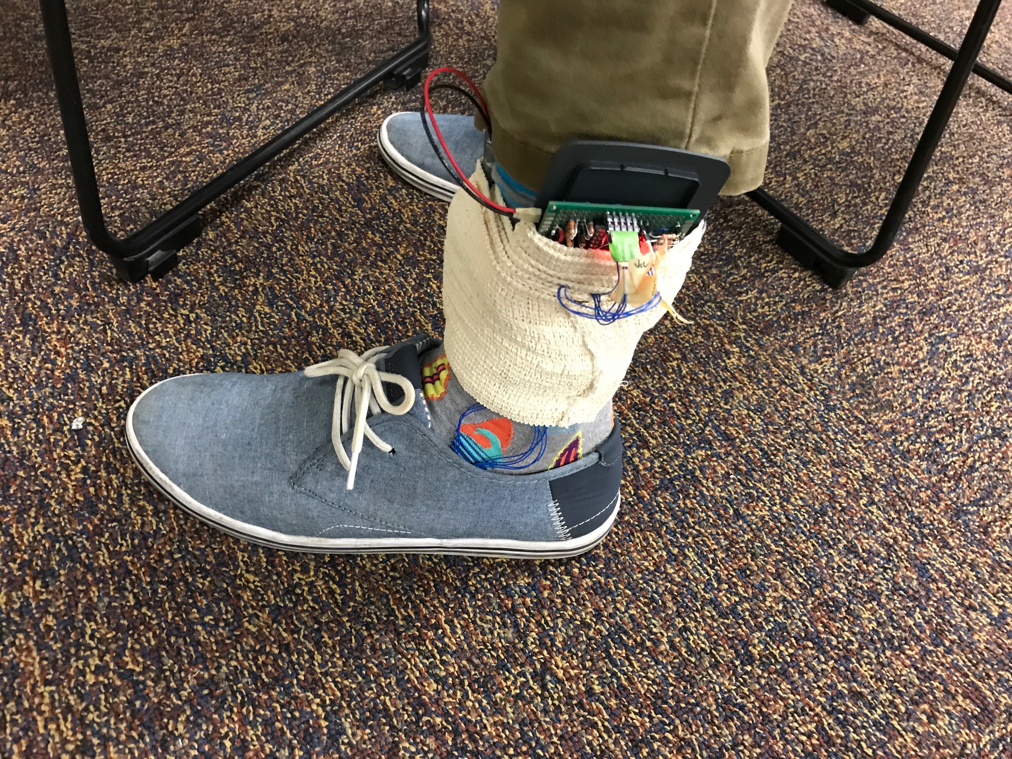The first prototype was fastened via medical wrap, and connected to sensors in the insole with thin wire.

My Responsibilities and Accomplishments

As team leader, I was most invested in the success of the team, and many times I had to fill in for the responsibilities of other team members when they were too busy with school work or other commitments. Aside from managerial tasks, I also contributed heavily to the software of the design.

Below list a few of my accomplishments and responsibilities:

• Team Leader
  • Recruited team members
  • Established team communication software and team document storage
  • Organized and scheduled team meetings
  • Created bi-weekly team progress presentations for the competition
  • Presented bi-weekly to competition organizers on team progress
  • Weekly task delegation to all 7 team members
  • Motivate and focus team members to facilitate productiveness
• Hardware
  • Soldering, debugging and rework of prototype.
  • Integrated serial bluetooth dongle into prototype
• Software
  • Established bluetooth firmware to publish live sensor data from prototype
  • Implemented multi-threaded software stack that would detect gait abnormalities in real time (below are the threads I implemented)
    • Bluetooth thread: Reads and stores live data from bluetooth connected prototype. Computation time: ~0.05 seconds
    • Inference thread: Takes chunks of live data of size N and processes it via forward propogation of a trained feed-forward neural network, and outputs whether or not the subject wearing the prototype is walking with a gait abnormality in real time. Computation time: ~0.2 seconds
    • Visualization thread: Visualizes the results of the rest of the stacks in GUI form.
  • Manually collected and labeled hours of walking/shuffling data to train the algorithm
  • Designed and implemented a feed-forward neural network to analyze live data from the prototype and infer whether the subject is walking with a gait abnormality.

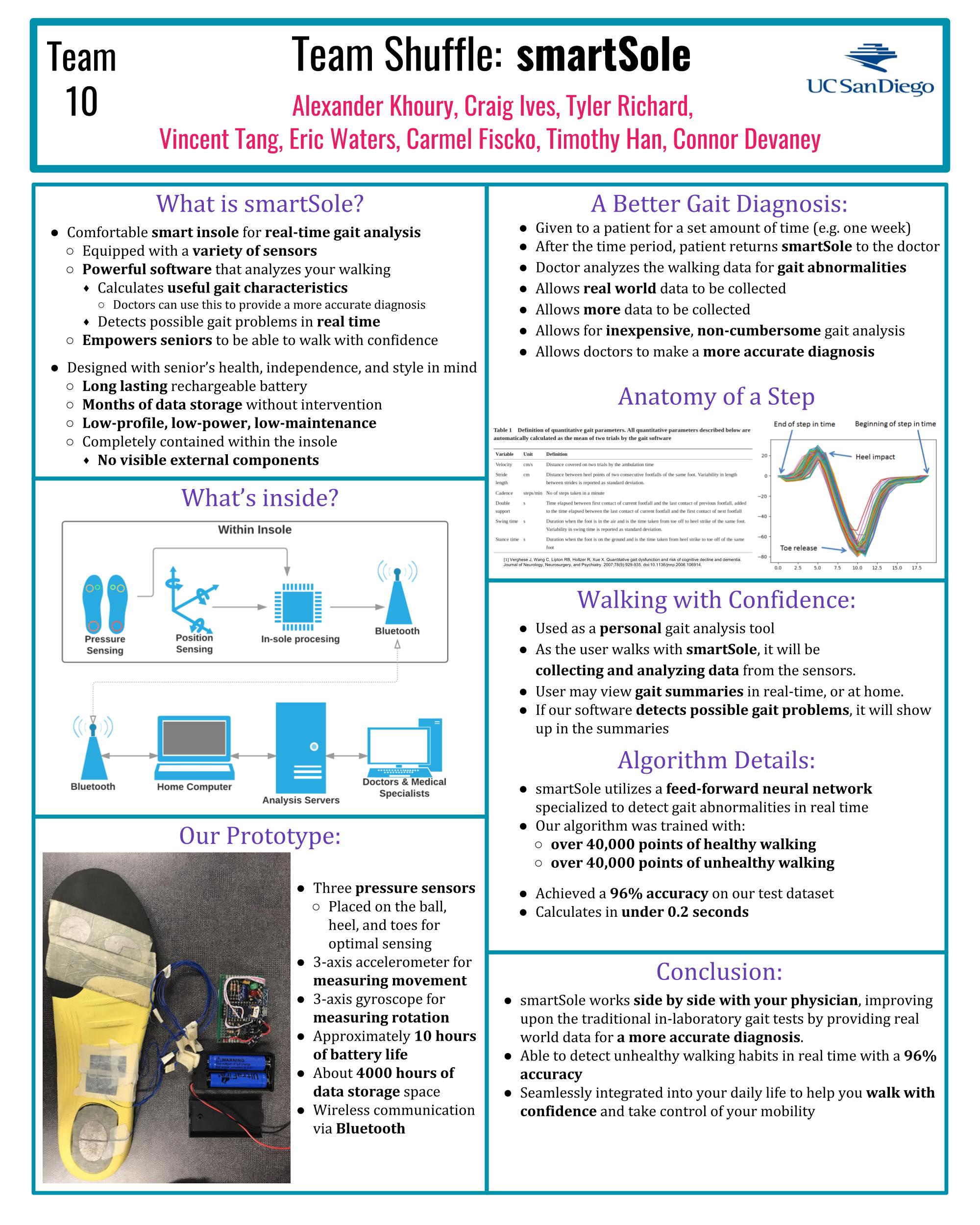
Poster

The poster was showcased at the design competition where our team members would answer any questions about the design of smartSole. Our booth also featured a live demo of the imu on the prototype.

The Competition

Below are a few pictures taken on competition day of our team. The competition consisted of a design showcase, as well as a 5 min presentation/demo of the design. During the presentation, we were able to have a successful demo of our prototype inferring between healthy and unhealthy walking on stage. The demo was not prerecorded, and the data collected was live from the prototype at the time at on stage. Showing this enabled us to achieve the popular vote by a large margin, winning us 2nd place. The reason I suspect we did not win 1st is we did not have as many interactions with senior citizens as the 1st place team (~45 compared to ~10), where facilitating senior-student interaction is a main goal of competition. Our development effort was focused into delivering a working prototype that would reflect our proposed design, and we succeeded, as we the only team to deliver a working protoype and demo it live.

(Video of a demo coming soon)

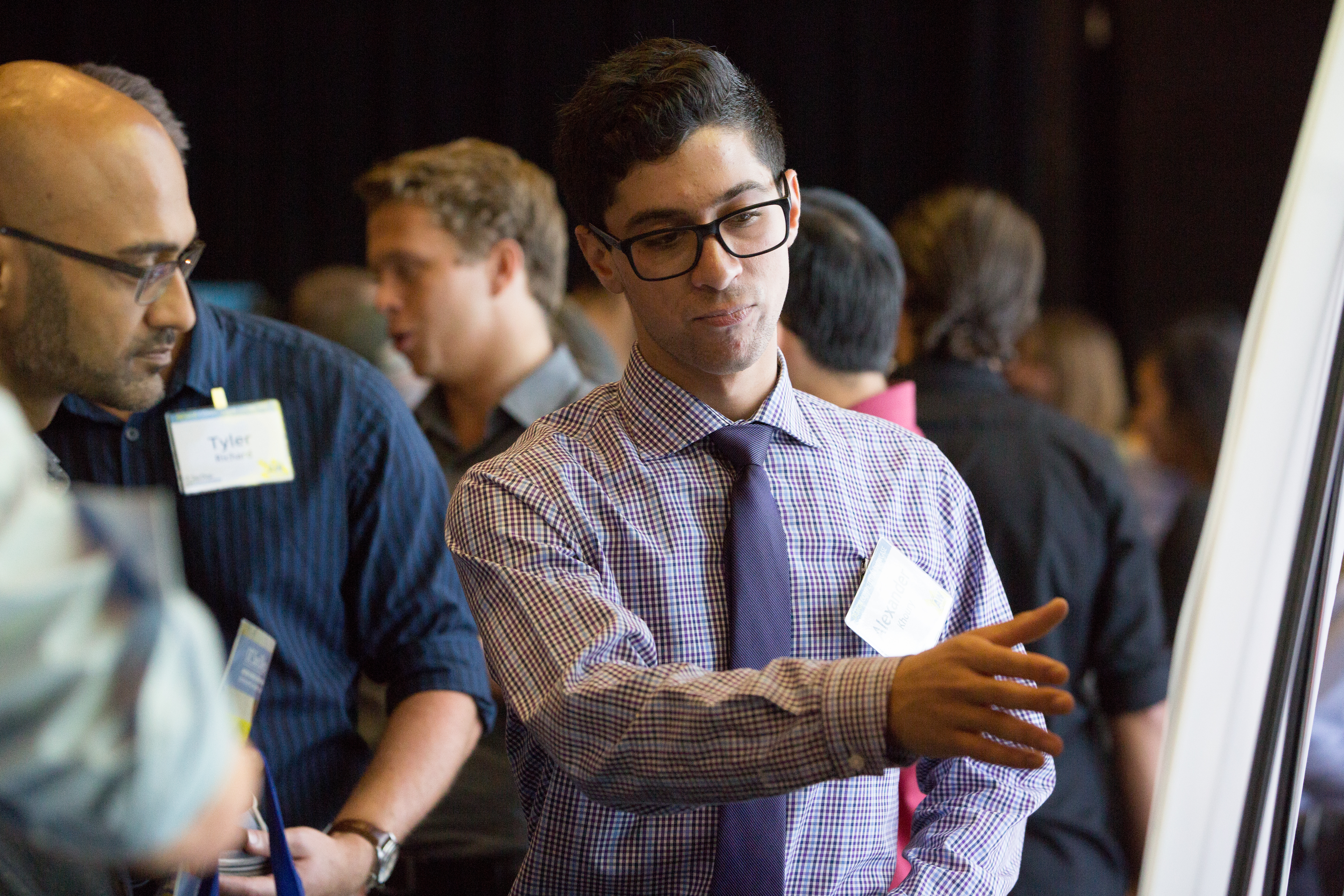The competition included showcasing our design, poster, and working prototype to anyone who came by.

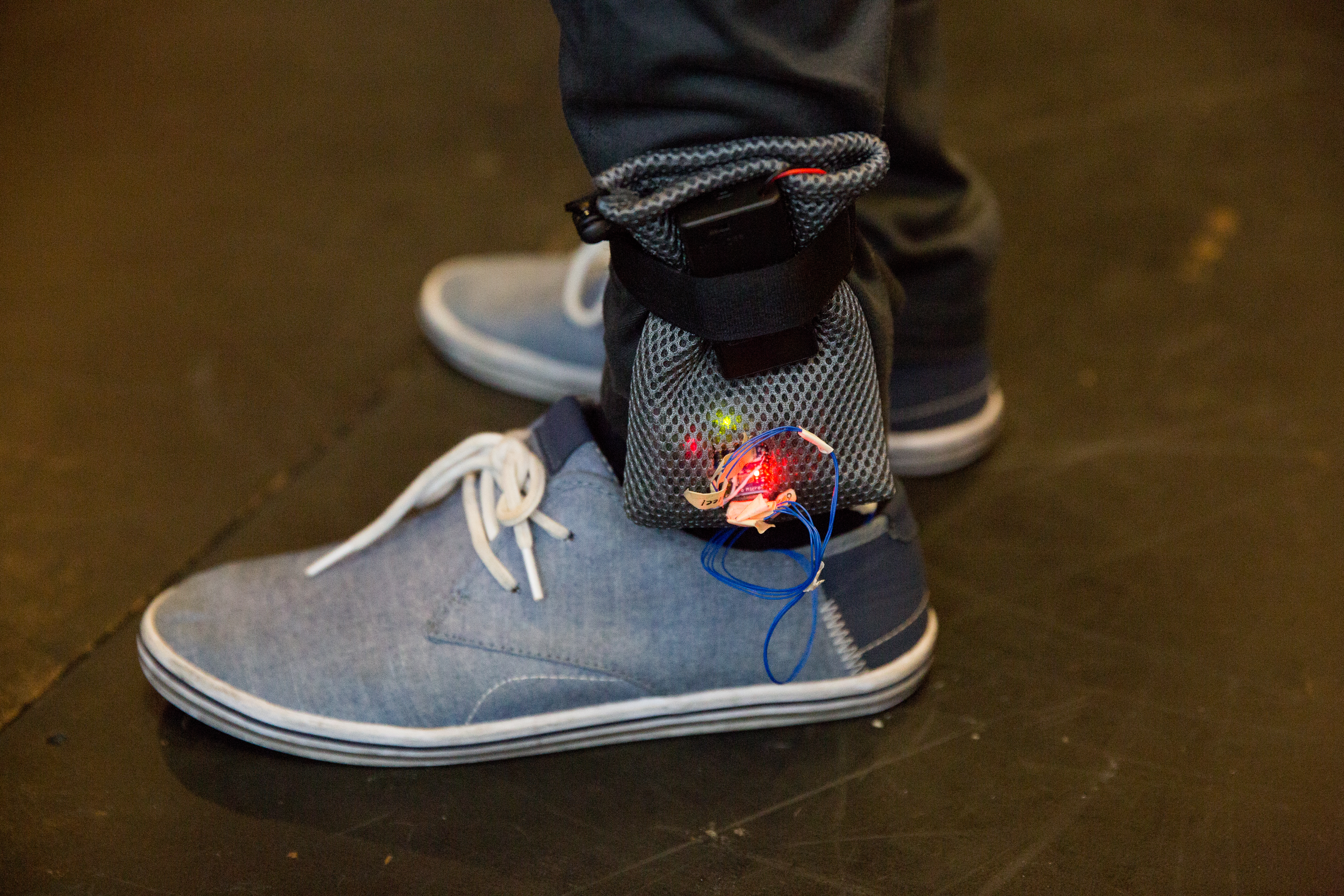This is the final prototype used on competition day.

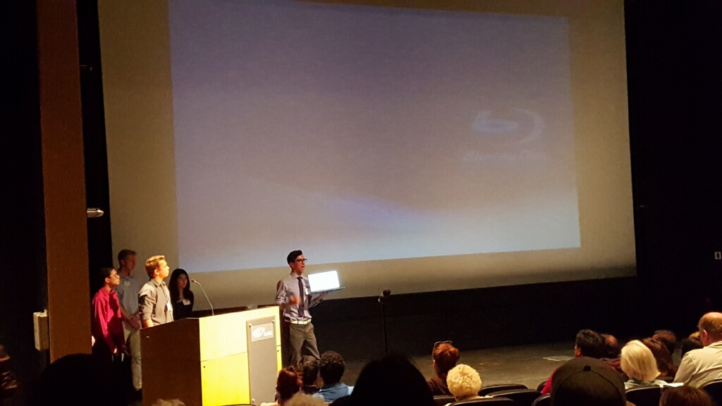Team Shuffle live demonstration, presentation day. We faced a technical difficulty during the presentation where the laptop used for the demo was unable to connect to the large screen, so unfortunately the demo was shown off of a laptop. Afterwards, and during, we worried that the laptop would make the demo too small to view in the auditorium; however, many audience members confronted me, complimenting me on our work, and saying that the demo was visible from where they were seated (off the laptop). Because of the use of colors in our visualization (green for healthy and orange for unhealthy), they were able to see the demo from a distance.

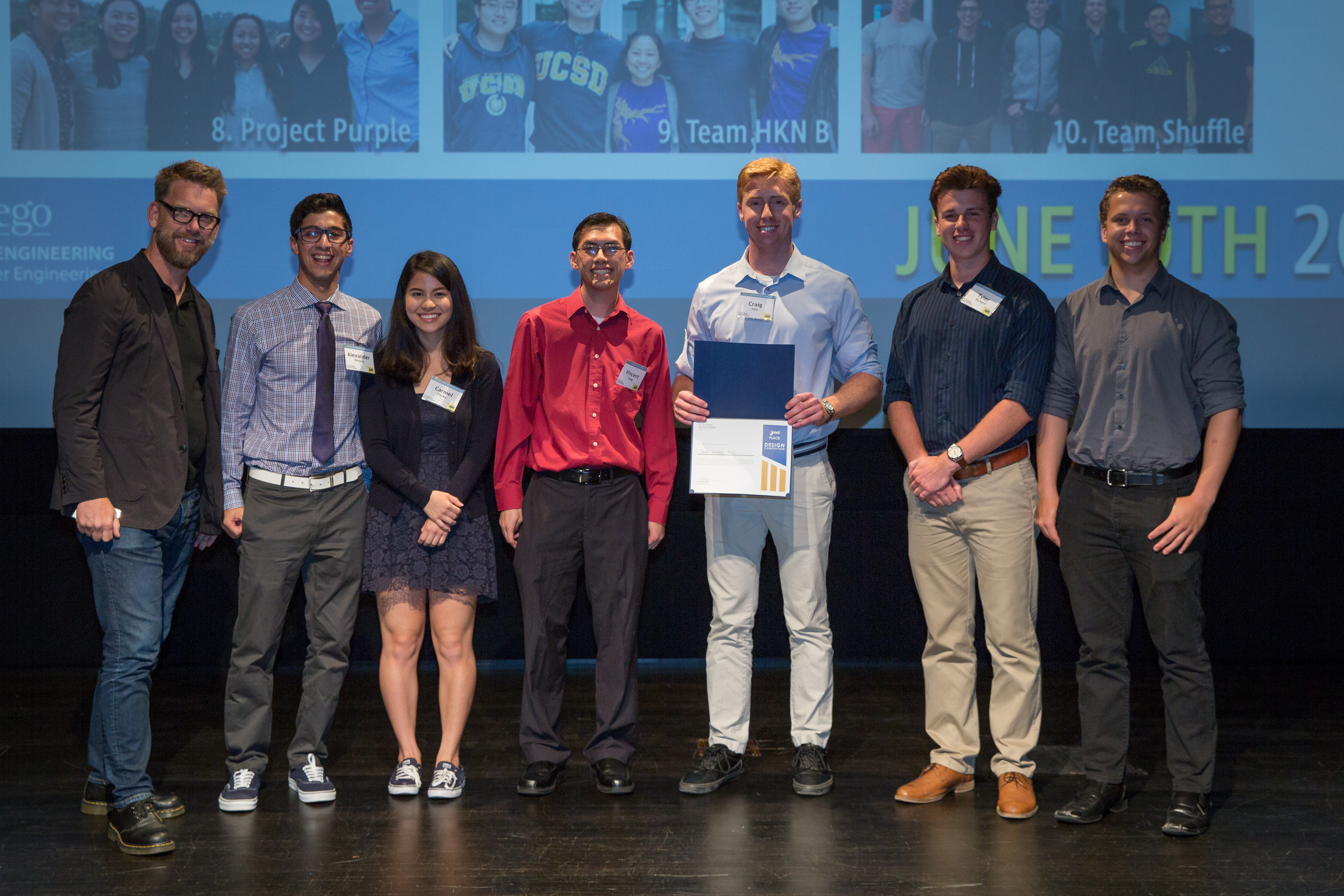Team Shuffle was awarded 2nd place in the competition, with a prize of $2000.

Feed Forward Neural Network

Network Structure

The structure that was chosen was a one hidden layer feed-forward neural network model (FNN). The input and hidden layer dimension sizes are of variable size, such that it allows for programmatic tuning of these dimensions to allow searching for an optimum network configuration. With this implementation, the output structure is fixed to the number of classes, such that we are able to train each node to activate with a specific class.

FNN structure with variable input and hidden layer dimension sizes

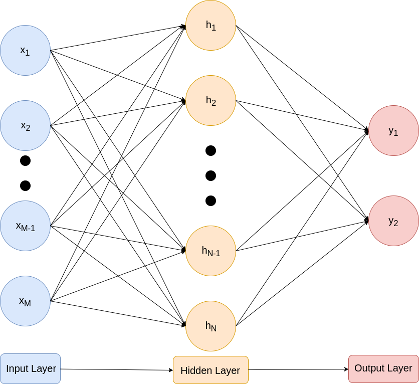
The equations describing the network from the inputs to the outputs:

$$\begin{equation} \begin{split} z_1 &= \sum_{i=1}^{M}{x_i \cdot W_i}+b\\ h &= tanh(z_1)\\ z_2 &= h \cdot W_h+b_h\\ \hat{y} &= softmax(z_2) \end{split} \end{equation}$$

The linear estimator to the hidden layer relies on a weighted sum over the inputs. This is fed into a tanh non-linear activation function, which in turn is the input to another linear estimator to the output layer. The softmax function at the output converts the resulting logits into probabilities per class.

Loss Function

This model was trained using a cross-entropy loss:

$$\begin{equation} L(y,\hat{y}) = -\dfrac{1}{T}\sum_{t = 1}^{T}\sum_{c = 1}^{C}y_{t,c} \cdot log(\hat{y}_{t,c}) \end{equation}$$

where $T$ is the number of training examples, and $C$ is the number of classes, which in our case is $2$, walking versus shuffling. The cross-entropy loss punishes on wrong guesses logarithmically proportional to the confidence of the model in the wrong guess itself.

Training

Stochastic Gradient Descent was used to train the model, allowing for flexibility in batch size, learning rate, and max iterations. In order to calculate the gradients for updating each parameter, the back propagation algorithm was used. Each parameter’s gradients would be calculated as follows:

$$\begin{equation} \begin{split} \dfrac{dL}{dW_h} &=\dfrac{dL}{d\hat{y}}\cdot\dfrac{d\hat{y}}{dz_2}\cdot\dfrac{dz_2}{dW_h}\\ \dfrac{dL}{db_h} &=\dfrac{dL}{d\hat{y}}\cdot\dfrac{d\hat{y}}{dz_2}\cdot\dfrac{dz_2}{db_h}\\ \dfrac{dL}{dW_i} &= \dfrac{dL}{d\hat{y}}\cdot\dfrac{d\hat{y}}{dz_2}\cdot\dfrac{dz_2}{dh}\cdot\dfrac{dh}{dz_1}\cdot\dfrac{dz_1}{dW_i}\\ \dfrac{dL}{db} &= \dfrac{dL}{d\hat{y}}\cdot\dfrac{d\hat{y}}{dz_2}\cdot\dfrac{dz_2}{dh}\cdot\dfrac{dh}{dz_1}\cdot\dfrac{dz_1}{db}\\ \end{split} \end{equation}$$

Data Preprocessing

The main preprocessing steps are summarized as follows:

1. Combine datasets

2. Isolate data sources selected as inputs

   When starting the algorithm, the user can specify the data sources to be used to train the model, such as combinations from Pitch, Yaw, Roll, Y-Acceleration, etc.

3. Reshape data into arrays of blocks (chunks)

   Each of these data sources begins as a 1-dimensional vector, it is necessary to reshape them a vector of chunks of specified width, chunk size, to feed into the network for classification. Because the resulting array is 2-dimensional, handling multiple inputs requires a 3-dimensional tensor structure to hold the data.

4. Generate one-hot labels

   Each of these chunks will require a one-hot label, defined as either the vector $[1, 0]$ for walking, or $[0, 1]$ for shuffling.

5. Shuffle data

   It is necessary to shuffle the data before the next preprocessing step, such as to include examples from each of the combined datasets in the training/validation sets. The labels are appended to the end of the chunks, such that the shuffling process preserves the labels.

6. Split into training and validation sets

   The data needs to be split in favor of a larger training than validation set, such that the networks accuracy can be tested on data it has not seen beforehand.

Model Implementation

For ease of implementation, the model was built and trained using Google’s TensorFlow. It was structured such that it could be iterated on over various vectors of parameters, and would save per iteration statistics and models.

FNN graphical model, using TensorFlow’s TensorBoard

Search for an Optimal Configuration

With building an adaptable model, parametric grid sweeps can be preformed to find an optimal configuration for the model. These parameters include the inputs selected, hidden layer dimension size, chunk size, batch size, and learning rate.\[1\baselineskip]

1. Input Selection

   To avoid exhaustive sweeps over 15+ data sources, intuition was used to narrow them down to a few for analysis. Pitch, all three acceleration axes, as well as the pressure data sources were considered. Among them, there were only two that gave high accuracy, Pitch, and X-Acceleration.

2. Hidden Layer Dimension Size, Chunk Size, Batch Size

   With less physical intuition to base off of, to find the optimal values for these parameters, 12 by 12 grid sweeps were preformed, recording accuracy on the validation set. The first of which was a sweep of hidden layer dimension size versus the chunk size. A higher hidden dimension size increases the complexity of the model, and increases the computation time of the network; however, having this parameter being larger, also dramatically increases the accuracy on our validation set. Also, having a larger chunk size means a longer real-time computation, as the network would have to wait for that chunk of data before processing. Batch size is an important factor in finding a global minimum in the loss function, as using a lower batch size will reduce the chance of the algorithm getting stuck in undesired local minima. A higher batch size will have more stable gradients, but takes more time to optimize.

\begin{figure}[H] \centering \includegraphics[width=.4\linewidth]{images/sweep1.png} \includegraphics[width=.42\linewidth]{images/sweep2.png}
\includegraphics[width=.4\linewidth]{images/sweep1.png} \textit{\caption{12x12 Sweeps}} \end{figure}

1. Learning Rate

   Learning rate is the proportionality of which to adjust the weights by the gradients. Too small of a learning rate will result in a large convergence time, but a large learning rate can put too much trust in a step in the wrong dimension.

2. Max Iterations

   It is important not to overfit the model onto the data, otherwise the performance on new data will be lower.

High accuracies, 90-93 percent, were found with many combinations of these parameters, but the most consistent higher accuracies, 93-96 percent, were found with the following parameters.

$$\begin{equation} \begin{split} \textbf{Optimal Configuration Summary: }\\ \textrm{Inputs Selected: }& \quad [Pitch,\space X-Acceleration]\\ \textrm{Hidden Layer Dimension: }& \quad 2000\\ \textrm{Chunk Size: }& \quad 20\\ \textrm{Batch Size: }& \quad 200\\ \textrm{Learning Rate: }& \quad 0.001\\\\ \textbf{Results Summary: }\\ \textrm{Training Examples: }& \quad 3487 \ chunks\\ \textrm{Validation Examples: }& \quad 1494 \ chunks\\ \textrm{Accuracy: }& \quad 0.96185\\ \textrm{Cross Entropy Loss: }& \quad 0.35213\\ \end{split} \end{equation}$$

Paper

Team Shuffle was formed in part to fulfill the graduation requirement of a senior design project. For more details about implementation please see our paper.